The Ultimate Guide to NGS Data Preprocessing Techniques
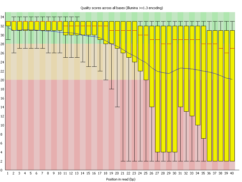
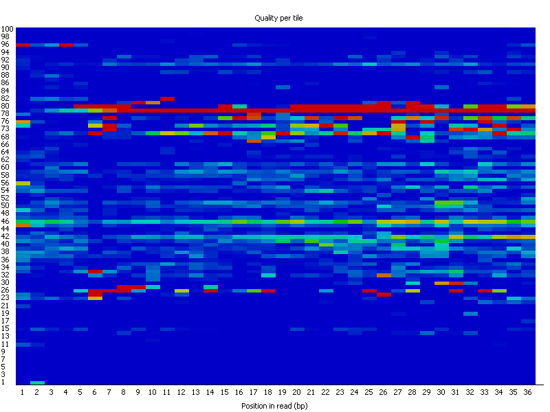
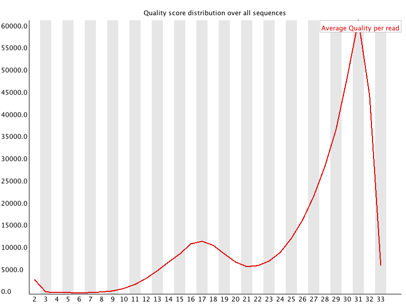
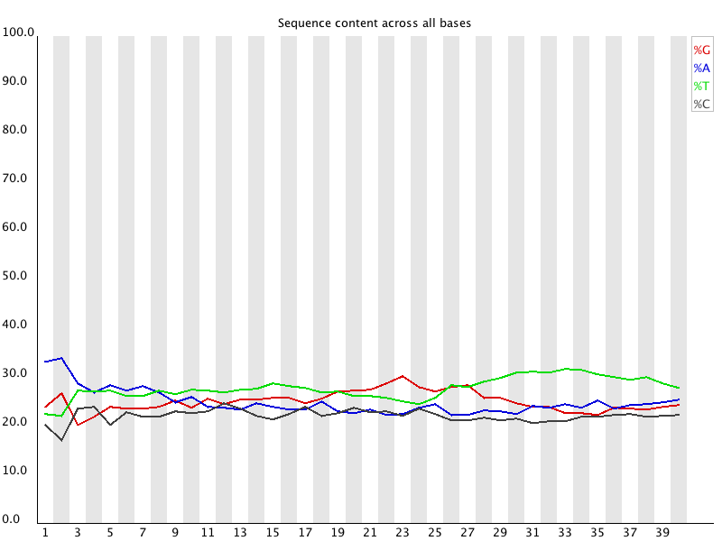
FASTQ files serve as the “raw data files” for any sequencing application, indicating that they are “unaltered.” Consequently, this file format is utilized for performing Quality Checks on sequencing reads. The Quality Check process is typically carried out using the FastQC tool developed by Simon Andrews from Babraham Bioinformatics. (https://www.bioinformatics.babraham.ac.uk/projects/fastqc/). FastQC and similar tools are instrumental in evaluating the overall quality of a sequencing run and are extensively employed in Next-Generation Sequencing (NGS) data production settings as an initial QC checkpoint. This tool offers a modular array of analyses that can provide a quick assessment of potential issues with your data that should be considered before proceeding with further analysis. The key features of FastQC include: • Importing data from *.bam, *.sam, or *.fastq files (any variant). • Delivering a swift overview to indicate areas that may present problems. Ideally, your FastQC report would appear as follows: Basic Statistics, Per base sequence quality, Per tile sequence quality, Per sequence quality scores, Per base sequence content, Per base GC content, Per base N content, Sequence Length Distribution, Sequence Duplication Levels, Overrepresented sequences, Adapter Content. However, since we do not exist in an ideal world, it is rare to receive such a report. FastQC reports feature summary graphs and tables that allow for a rapid evaluation of your data. At the top of the FastQC HTML report, you will find a summary of the modules that were executed, along with a brief assessment of whether the results from each module appear to be completely normal (indicated by a green tick), somewhat abnormal (shown by an orange triangle), or highly unusual (marked with a red cross). In detail, you will receive graphs for all the modules listed above, providing insights into the quality of your input data. This module provides fundamental details regarding the input FASTQ file: its name, the type of quality score encoding, the overall number of reads, the length of the reads, and the GC content. It includes: The Basic Statistics module produces straightforward compositional statistics for the analyzed file. Filename: The initial name of the file that was analyzed, File type: Indicates whether the file contained actual base calls or colorspace data that needed conversion to base calls, Encoding: Specifies which ASCII encoding of quality values was detected in this file, Total Sequences: A tally of the total sequences processed. Two figures are reported: actual and estimated. Currently, these values will always match. In the future, it may be feasible to analyze only a subset of sequences and estimate the total to expedite the analysis. However, since problematic sequences are not uniformly distributed throughout a file, this feature has been disabled for now, Filtered Sequences: When operating in Casava mode, sequences marked for filtering will be excluded from all analyses. The count of such removed sequences will be indicated here. The total sequences count mentioned above will not account for these filtered sequences, reflecting only the number of sequences actually utilized in the further analysis, Sequence Length: Displays the lengths of the shortest and longest sequences in the dataset. If all sequences share the same length, only one value will be shown, %GC: The overall %GC of all bases across all sequences. Basic Statistics does not generate warnings, Basic Statistics does not produce errors, This module does not issue warnings or errors. This box-and-whisker diagram illustrates the range of quality scores across all bases at each position within the FASTQ file. The central red line signifies the median score, while the yellow box indicates the inter-quartile range (25–75%). The upper and lower whiskers represent the 10% and 90% points respectively, and the blue line denotes the average quality. On the x-axis, the bases 1–10 are displayed individually, followed by a summary of the bases grouped into bins. The quantity of base positions grouped together varies based on the read length, meaning shorter reads will have narrower windows and longer reads will have wider windows. The y-axis presents the Phred-Scores. It is common to observe a decline in quality as the base position increases. This phenomenon is attributed to Illumina's sequencing by synthesis technology and is referred to as phasing. During each sequencing cycle, chemicals containing variants for all four nucleotides are applied to the flow cell. Each nucleotide is capped with a terminator, allowing only one base to be incorporated at a time. After the fluorescence signal is detected, the terminator cap is removed, enabling the next cycle to commence. As a result, synchronized sequencing of DNA fragments in each cluster is achieved through the expression of specific fluorescence signals. The primary cause of the diminishing sequence quality is the improper removal of the nucleotide blocker after signal detection (phasing), which leads to light interference during signal detection. This error becomes more frequent over time and as the read length increases. The Per tile Sequence Quality Graph will only show up in your FastQC report if you are utilizing an Illumina library. The initial sequence identifiers are preserved, reflecting the flowcell tile from which each read originated. Errors on this plot may arise from temporary issues like bubbles moving through the flow cell, or they might be indicative of more lasting problems such as smudges on the flowcell or debris present within the flow cell lane. This graph depicts the overall count of reads in relation to the average sequence quality score for each complete read, enabling the identification of whether a portion of your sequences has consistently low quality. In subsequent data analysis phases, only a minimal fraction of the total sequences should exhibit poor quality. The graphs shown below illustrate the percentage of bases identified for each of the four nucleotides (A/T/G/C) at every position across all reads in the FASTQ file. Once more, the x-axis is not consistent as previously mentioned for the per-base sequence quality. In a typical sequencing library, one would anticipate minimal variation between the different bases in a sequencing run, meaning the lines in this graph should run parallel to one another. If significant biases are observed that vary with different bases, this is often linked to contamination in your library due to overrepresented sequences, such as clonal reads or adapters. It is important to note that in DNA-Seq libraries, the ratio of each base tends to remain fairly stable throughout the length of a read; however, most RNA-Seq libraries display an uneven distribution of bases for the initial 10-15 nucleotides. This is considered normal and expected. The per base GC content graph displays the GC composition at each base position within a file. In a random library, this graph should appear as a horizontal line. A consistent bias across all base positions suggests that the original library was biased towards certain sequences or points to a systematic issue during the sequencing process. A varying GC bias across different bases, on the other hand, suggests contamination with overrepresented sequences. This graph shows the number of reads plotted against the GC content of each read in percentage. In DNA sequencing, all reads should ideally create a normal distribution, with the peak aligning with the mean GC content of the organism being sequenced. In RNA sequencing methods, there might be a variation in the distribution of mean GC content among transcripts, as illustrated in the graph. A shifted normal distribution signifies a systematic bias that is independent of base position. This graph represents the percentage of bases at each position in a read that are designated as “N” (no base call). If the curve noticeably rises above zero at any position, it indicates an issue during the sequencing run. As shown in the report, the sequencing instrument failed to call a base for approximately 20% of the reads at position 29. Typically, a low occurrence of Ns is found towards the end of a sequence. For short-read sequencing, fragments of consistent length should be produced based on your sequencing parameters (50 bp, 75 bp, 100 bp, 150 bp). However, this length may vary after trimming sequences from the ends due to low-quality base calls or adapter contamination. If long-read sequencing was conducted, you will see a variety of read lengths, implying that while some reads are shorter, most have a concentrated size distribution, with some being longer. There are two origins of duplicate reads: PCR duplication resulting from biased PCR enrichment or truly overrepresented sequences, such as highly abundant transcripts in an RNA-Seq library. PCR duplicates distort the actual proportion of sequences present in the starting material, while genuinely overrepresented sequences accurately reflect your input. Therefore, in DNA-Seq, nearly all reads should be unique, whereas in RNA-Seq, duplicates of highly abundant transcripts may occur, and such duplication is considered normal in this context. In a random library, it is anticipated that the majority of sequences will appear only once in the final collection. This module identifies all sequences that are present more frequently than anticipated. Discovering that a particular sequence is overrepresented can indicate either significant biological importance or contamination within the library. For each identified overrepresented sequence, the program searches for matches in a database of common contaminants and will report the most relevant result it finds. Frequently, adapter sequences are identified as overrepresented reads. This situation may arise when using a long read length, and some of the library inserts are shorter than the read length, causing the read to extend into the adapter at the 3’ end. Guidance on how to eliminate adapter sequences is provided. Moreover, you can also perform quality trimming with sequences depicting a bad phred score. This can be done with the additional option cutadapt - to trim low-quality bases from 5’ and/or 3’ ends of each read before adapter removal. Applied to both reads if data is paired. If one value is given, only the 3’ end is trimmed. If two comma-separated cutoffs are given, the 5’ end is trimmed with the first cutoff, the 3’ end with the second. Find some more options in terms of the command cutadapt by cutadapt - - help. Another tool for adapter trimming or removal of low-quality bases is flexbar. Demultiplex raw BCLs → FASTQ (check sample sheet). Initial QC with FastQC and aggregate with MultiQC. Adapter & quality trimming (e.g., cutadapt, fastp, Trimmomatic; keep ≥Q20–30, MINLEN ~30–50). Contaminant removal (rRNA/host/adapters with BBDuk or Bowtie2; optional taxon screen with Kraken2). Dedup/UMI handling (mark duplicates after alignment or use UMI-tools before counting). Post-trim QC (re-run FastQC/MultiQC to confirm improvements). Trim adapters (yes) and very low-quality tails (usually yes). Modern aligners soft-clip, but leftover adapters and long low-Q tails reduce mapping quality and inflate false positives. Use minimal, conservative trimming (e.g., cutadapt -q 20,20 -m 30 for PE reads), avoid over-trimming that shortens reads excessively, and always compare pre/post alignment metrics. Per-base sequence quality: should stay >Q20; a steady decline at the 3′ end is common. Adapter content / Overrepresented sequences: typically adapters or primers—address with trimming. Per-sequence GC content: big shifts suggest bias or contamination (metagenomes and RNA-seq can deviate). Per-base sequence content: failing in the first 10–15 nt is normal for many RNA-seq libraries (random hexamer bias). Focus on these modules first; use MultiQC to track changes across samples after trimming/filtering. 1. FastQC Help Index and Documentation – https://www.bioinformatics.babraham.ac.uk/projects/fastqc/Help/ 2. MultiQC Overview – https://multiqc.info/ 3. Illumina Q-score Explanation – https://emea.support.illumina.com/bulletins/2016/04/what-is-a-q-s core-and-how-do-you-interpret-q-scores-in-sequencing.html 4. Illumina Technical Note on Quality Scores – https://www.illumina.com/documents/products/technotes/technote_Q-Scores.pdf 5. fastp Paper – Chen et al., 2018, Bioinformatics, https://doi.org/10.1093/bioinformatics/bty560 6. fastp Documentation – https://github.com/OpenGene/fastp 7. Cutadapt Documentation – https://cutadapt.readthedocs.io/ 8. Cutadapt Adapter Trimming Recipes – https://cutadapt.readthedocs.io/en/stable/guide.html 9. Trimmomatic Manual – http://www.usadellab.org/cms/?page=trimmomatic 10. Illumina Adapter Sequences (i5/i7 orientation caveats) – https://support-docs.illumina.com/SHA RE/AdapterSeq/Content/SHARE/AdapterSeq/AdapterSeqIntro.htm 11. FastQ Screen Documentation – https://www.bioinformatics.babraham.ac.uk/projects/fastq_screen/ 12. FastQ Screen Paper – Wingett & Andrews, 2018, F1000Research, https://doi.org/10.12688/f1000research.15931.2 13. Kraken2 Paper – Wood et al., Genome Biology, 2019, https://doi.org/10.1186/s13059-019-1891-0 14. BBduk (BBTools) Documentation – https://jgi.doe.gov/data-and-tools/software-tools/bbtools/ 15. Illumina PhiX Control Guide – https://www.illumina.com/products/by-type/sequencing-kits/cluste r-gen-sequencing-reagents/phix-control-v3.html 16. GATK Discussion on Quality Trimming – https://gatk.broadinstitute.org/hc/en-us/articles/360035531112 17. UMI-tools Paper – Smith et al., 2017, Genome Research, https://doi.org/10.1101/gr.209601.116 18. UMI-tools Documentation – https://umi-tools.readthedocs.io/ 19. RSeQC Documentation – http://rseqc.sourceforge.net/ 20. RSeQC Paper – Wang et al., 2012, Bioinformatics, https://doi.org/10.1093/bioinformatics/bts356 21. RNA-SeQC 2 Paper – Graubert et al., 2021, Bioinformatics, https://doi.org/10.1093/bioinformatics/btab305 22. Qualimap RNA-seq Module – http://qualimap.conesalab.org/ 23. Picard CollectRnaSeqMetrics – https://broadinstitute.github.io/picard/ 24. SortMeRNA Paper – Kopylova et al., 2012, Bioinformatics, https://doi.org/10.1093/bioinformatics/bts611 25. iVar Documentation – https://andersen-lab.github.io/ivar/html/ 26. nf-core/viralrecon Pipeline Documentation – https://nf-co.re/viralrecon 27. ARTIC Network SARS-CoV-2 Primer Scheme – https://artic.network/ncov-2019 28. ONT Dorado Basecalling – https://github.com/nanoporetech/dorado 29. pycoQC Paper – Leger & Leonardi, 2019, Journal of Open Source Software, https://doi.org/10.21105/joss.01236 30. NanoPlot Documentation – https://github.com/wdecoster/NanoPlot 31. Filtlong Documentation – https://github.com/rrwick/Filtlong 32. Porechop (archived) – https://github.com/rrwick/Porechop 33. Porechop_ABI (2023) – https://github.com/a-slide/Porechop_ABI 34. PEAR Paper – Zhang et al., 2014, Bioinformatics, https://doi.org/10.1093/bioinformatics/btt593 35. BBMerge Paper – Bushnell et al., 2017, PLOS One, https://doi.org/10.1371/journal.pone.0185056 36. AdapterRemoval v2 Paper – Schubert et al., 2016, BMC Research Notes, https://doi.org/10.1186/s13104-016-1900-21. Introduction
2. The Basic Statistics Module
3. Per Base Sequence Quality
4. Per Tile Sequence Quality
5. Per Sequence Quality Scores
6. Per Base Sequence Content
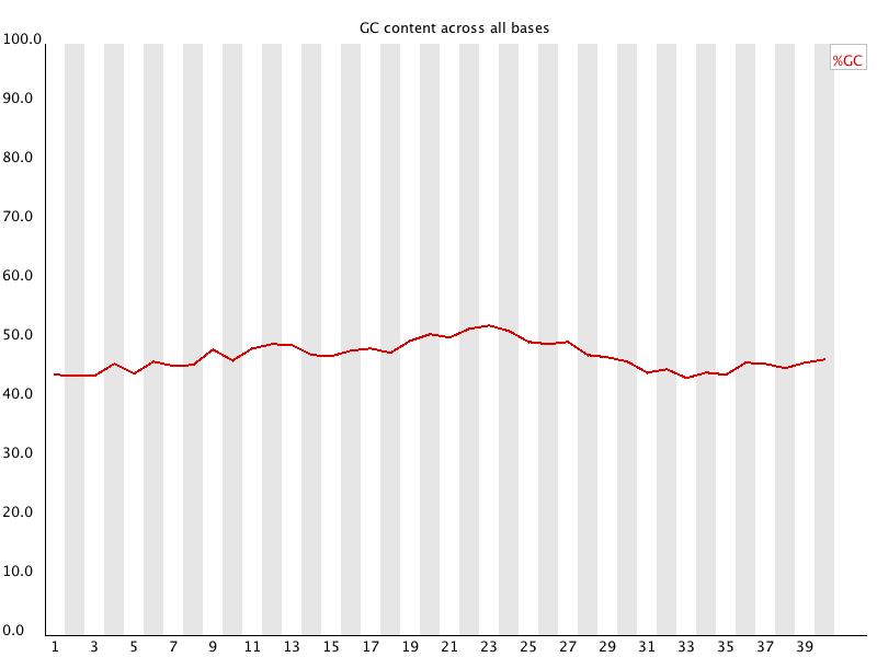
7. Per Base GC Content
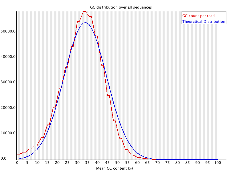
8. Per Sequence GC content
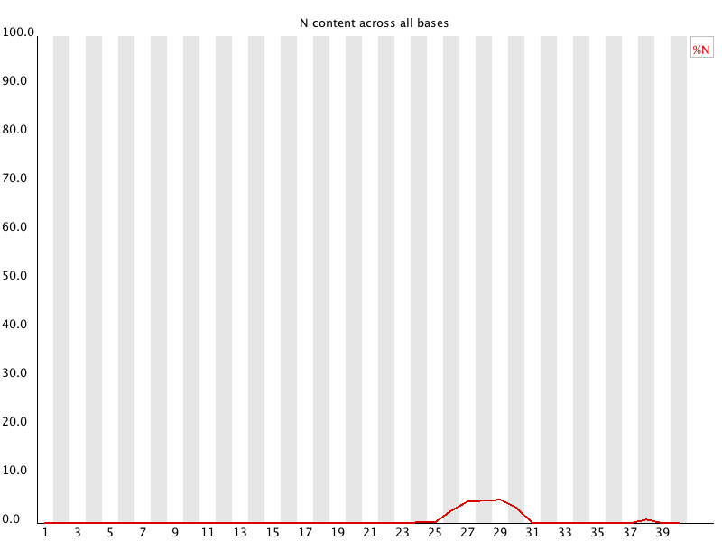
9. Per Base N Content
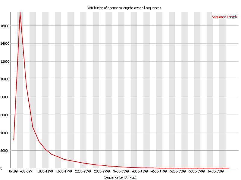
10. Sequence Length Distribution
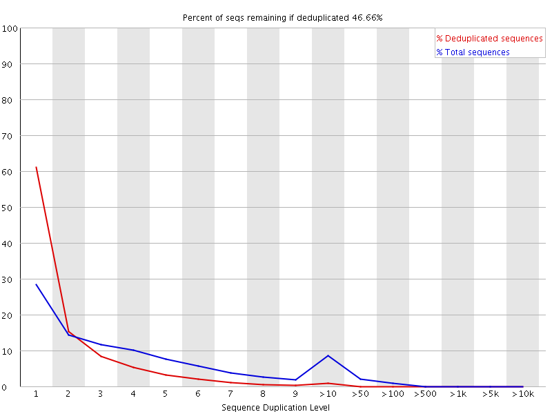
11. Sequence Duplication Levels
12. Overrepresented Sequences
13. Understanding the Adapter Clipping in NGS Data
14. FAQs
1. What are the core steps in NGS data preprocessing?
2. Should I always trim before alignment?
3. How do I read a FastQC/MultiQC report—what warnings matter most?
15. References for further reading
Recent Posts
FASTQ files serve as the “raw data files” for any sequencing application, indicating that they are “unaltered.” Consequently, this file format is utilized for performing Quality Checks on sequencing reads. The Quality Check process is typically carried out using the FastQC tool developed by Simon Andrews from Babraham Bioinformatics.
FASTA format is a text-oriented format utilized for depicting either nucleotide sequences or peptide sequences, where nucleotides or amino acids are denoted by a single-letter code.
Mammalian expression systems enable the production of complex, functional recombinant proteins with proper folding and post-translational modifications. These systems are ideal for studying human proteins in a near-native environment, offering advantages in scalability, gene delivery, and purification. HEK293 and CHO cells remain the most widely used hosts, supporting both transient and stable expression strategies for academic and pharmaceutical applications.
Gas Chromatography (GC) stands as one of the most powerful and versatile analytical techniques used to separate and analyze compounds in complex mixtures. At its core, GC enables the identification and quantification of chemical substances based on their molecular composition and retention behaviors during migration through a chromatographic column.
Calcium plays a crucial role as a specific cation, Ca2+, in cellular functions. It is expelled by all cell cytoplasm either into the extracellular environment or into internal reservoirs. From these reserves, it is discharged by stimuli from outside eukaryotic cells into the cytoplasm and organelles, where it triggers numerous processes.